Basic Data Input in Excel
Table of Contents
- Inputting data
- Identifying cells
- Cell ranges
- Entering formulas
- Relative versus absolute cell references
- Formatting cells
Introduction
Excel is a type of computer program called a spreadsheet.
It is probably the most widely used program for the management and analysis
of numeric data. The utility of Excel and other spreadsheet programs
comes from its visual method of storing and management of data. Each
unique bit of data is held in a cell. Each cell has a unique
location and can be referenced to format the display of the numeric
data, create graphs, and perform mathematical operations on the data.
Inputting data
You can enter data by simply clicking on one of the cells in the
spreadsheet and typing in your values. Normally you will start
entering somewhere near the upper left corner of the spreadsheet. You
can move to the next cell in a number of ways:
- Clicking on the next cell you want to enter data into
- Return will move to the next cell down
- Tab will move to the next cell to the right
- Arrow keys will move in the direction of the arrow
Referring to the figure below, the first row of data might be entered:
1 Tab 52 Tab 48 Tab 73.5
The first column might be entered:
1 Return 3 Return 2 Return 5 Return 2
Data in a cell can be deleted by highlighting a cell and either
typing in a new value or hitting Delete.
Return to Top
Identifying cells
Each cell is located in a rectilinear grid of
cells and is located by a column and row designation. Columns
are designated by letters while rows are designated
by numbers.
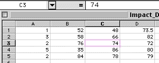
In this piece of an Excel spreadsheet, the number 74 is located
in cell C3. Notice that the location designation of the highlighted
cell is shown on the right of the first tool bar above the spreadsheet
(called the formula bar). Similarly, the value of the cell is also
shown in the formula bar. Every other number in this spreadsheet can be
located with a unique letter-number designation.
Return to Top
Cell ranges
Groups of cells can also be specified by placing a colon between the
upper left and lower right corners of the group of cells. For example:
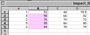
This highlighted column of cells would be B1:B5. Notice that the
letter designation is the same for a single column of cells. Another selection
might be:

Here, multiple rows and columns are selected and
would be designated as A2:C4.
Return to Top
Entering formulas
The power of spreadsheets is not just in being
able to hold numbers, but also manipulating them with mathematical formulas.
A cell is designated as having a formula in it by typing an equal
(=) sign as the first character. Next comes a combination
of cell designations and/or standard mathematical operators (+,
-, *, /) and/or special predefined functions. For
example:
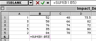
A formula is entered in cell B6, starting with the equal
sign followed by the special function SUM(). The cells to
be summed are specified inside the parentheses. In this case cells B1
to B5 are summed. The entry of B1:B5 into the function could
have been done by typing the letters or by clicking and dragging
on the range of cells of interest. Note that the formula is also shown
up in the formula bar. You can accept the formula either by typing return
or by clicking on the green checkmark to the left of the formula.
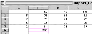
Cell B6 now shows the result of the formula calculation:
A complete list of functions can be found by clicking on a cell and choosing
Insert>Function...
Return to Top
Relative versus absolute cell references
Most formulas are applied numerous times to different
groups of cells, referring to a different range of cells each time it
is used in a different cell location. Because of this, Excel provides
a behavior to speed the updating of cell references. Supposed you had
your SUM formula entered in B6 and you wanted to use it to sum the values
in column C. You might select B6, choose Edit>Copy,
select C7, and choose Edit>Paste:
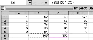
Notice up in the formula bar that the SUM function
now operates on C1:C5. When the formula was copied over one column
(B6 to C6), the range of cells referred to in the function
also shifted one column (B1:B5 to C1:C5). This is because
the cell references in the function were relative references.
If you do not want the cell(s) that a formula
refers to shift relative to where the formula is copied, you must use
absolute references. You can do so by putting a dollar ($)
sign before the letter and number in the cell designation. For example,
say your formula refers to a constant located in cell E7:
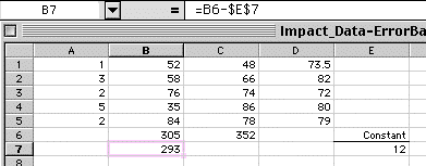
If you had simply entered the cell reference as E7, when the formula
in B7 was copied to C7, the reference to E7 would
have shifted to F7. This would be undesirable. Instead the constant
is referenced with $E$7. Now when it is copied:
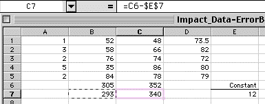
The formula in C7 still refers to cell E7.
Return to Top
Formatting cells
Often when data are inputted into cells, the numeric
values are not formatted the way you would like them to appear in the
spreadsheet or in graphs you will later create. The number of decimal
places, along with many other formatting options can be set by selecting
the cell or cells you would like to format and choosing Format>Cells...
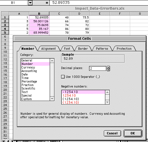
When you first click on the Number tab, your cells will be listed
in the Category General. This is the default data category for a new spreadsheet.
To control the decimal places, you will need to change the Category
to Number. Now type or click the arrows to
set the appropriate number of Decimal places. A preview of what
your formatted cell(s) will look like is shown in the Sample box.
You can also control how Negative numbers appear. For scientific
applications, you usually leave it at the default seen here.
Though in this example, the number of decimal places has been changed
to two places, the underlying value stored in the spreadsheet has not
been rounded:
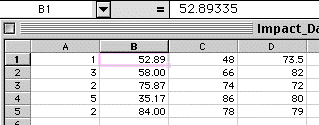
Note for the highlighted cell, the full five decimal places still show
up in the formula bar.
The number of decimal places can also be controlled with the tool bar
icons:

Return to Top
|


