The knowledge that any individual measurement
you make in a lab will lack perfect precision often leads a researcher
to choose to take multiple measurements at some independent variable
level. Though no one of these measurements are likely to be more precise
than any other, this group of values, it is hoped, will cluster
about the true value you are trying to measure. This distribution of
data values is often represented by showing a single data point, representing
the mean value of the data, and error bars to represent
the overall distribution of the data.
Let's take, for example, the impact energy absorbed
by a metal at various temperatures. In this case, the temperature of
the metal is the independent variable being manipulated by the researcher
and the amount of energy absorbed is the dependent variable being recorded.
Because there is not perfect precision in recording this absorbed energy,
five different metal bars are tested at each temperature level. The
resulting data (and graph) might look like this:
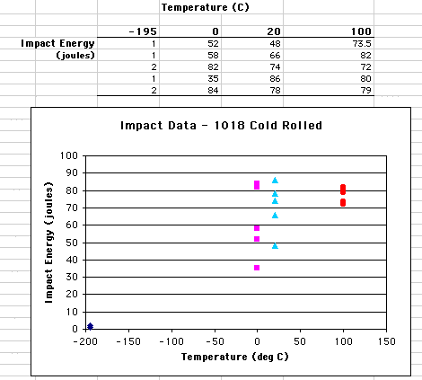
For clarity, the data for each level of the independent
variable (temperature) has been plotted on the scatter plot in a different
color and symbol. Notice the range of energy values recorded at each
of the temperatures. At -195 degrees, the energy values (shown in blue
diamonds) all hover around 0 joules. On the other hand, at both 0 and
20 degrees, the values range quite a bit. In fact, there are a number
of measurements at 0 degrees (shown in purple squares) that are very
close to measurements taken at 20 degrees (shown in light blue triangles).
These ranges in values represent the uncertainty in our measurement.
Can we say there is any difference in energy level at 0 and 20 degrees?
One way to do this is to use the descriptive statistic, mean.
The mean, or average, of a group of values describes
a middle point, or central tendency, about which data points vary. Without
going into detail, the mean is a way of summarizing a group of data
and stating a best guess at what the true value of the dependent variable
value is for that independent variable level. In this example, it would
be a best guess at what the true energy level was for a given temperature.
The above scatter plot can be transformed into a line graph showing
the mean energy values:
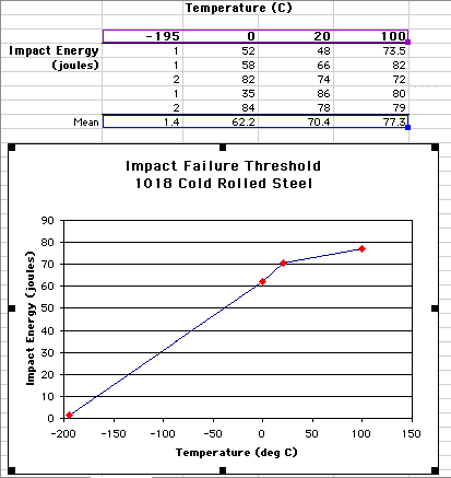
Note that instead of creating a graph using all of the raw data, now only the
mean value is plotted for impact energy. The mean was calculated for each temperature
by using the AVERAGE function in Excel. You use this function by typing =AVERAGE
in the formula bar and then putting the range of cells containing the data you
want the mean of within parentheses after the function name, like this:
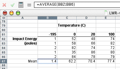
In this case, the values in cells B82 through
B86 are averaged (the mean calculated) and the result placed in cell
B87. Once you have calculated the mean for the -195 values, then copy
this formula into the cells C87, etc. If you look back at the line graph
above, we can now say that the mean impact energy at 20 degrees is indeed
higher than the mean impact energy at 0 degrees. However, though you
can say that the means of the data you collected at 20 and 0 degrees
are different, you can't say for certain the true energy values
are different. Can we ever know the true energy values? No, but you
can include additional information to indicate how closely the means
are likely to reflect the true values. You can do this with error
bars.
There are two common ways you can statistically
describe uncertainty in your measurements. One is with the standard
deviation of a single measurement (often just called the standard
deviation) and the other is with the standard deviation of
the mean, often called the standard error. Since
what we are representing the means in our graph, the standard error
is the appropriate measurement to use to calculate the error bars. While
we were able to use a function to directly calculate the mean, the standard
error calculation is a little more round about. First you have to calculate
the standard deviation with the STDEV function. It is used much
the same way AVERAGE was:
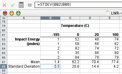
The standard error is calculated by dividing the
standard deviation by the square root of number of measurements that
make up the mean (often represented by N). In this case, 5 measurements
were made (N = 5) so the standard deviation is divided by the square
root of 5. By dividing the standard deviation by the square root of
N, the standard error grows smaller as the number of measurements (N)
grows larger. This reflects the greater confidence you have in your
mean value as you make more measurements. You can make use of the of
the square root function, SQRT, in calculating this value:
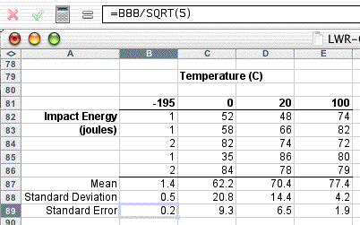
Using words you can state that, based on five
measurements, the impact energy at -195 deg C is 1.4 +/- 0.2 joules.
The +/- value is the standard error and expresses how confident you
are that the mean value (1.4) represents the true value of the impact
energy. Graphically you can represent this in error bars.
With the standard error calculated for each temperature,
error bars can now be created for each mean. First click the
line in the graph so it is highlighted. Now select Format>Selected
Data Series...
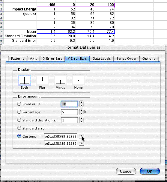
Select the Y Error Bars tab and then choose
to Display Both (top and bottom error bars).
Now click on the Custom button
as the method for entering the Error amount. You will want to
use the standard error to represent both the + and the -
values for the error bars, B89 through E89 in this case. Note:
it is critical to highlight the standardard deviation values for all
of the temperatures. This way the unique standard error value is associated
with each mean. The easiest way to do this is to click on the up arrow
button as shown in the figure above. The dialog box will now shrink
and allow you to highlight cells representing the standard error values:
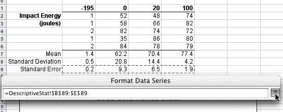
When you are done, click on the down arrow button
and repeat for the other value cell. When you are done, click OK.
Your graph should now look like this:
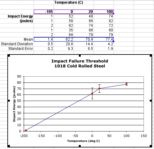
The error bars shown in the line graph above represent
a description of how confident you are that the mean represents the
true impact energy value. The more the orginal data values range above
and below the mean, the wider the error bars and less confident you
are in a particular value. Compare these error bars to the distribution
of data points in the original scatter plot above.Tight distribution
of points around 100 degrees - small error bars; loose distribution
of points around 0 degrees - large error bars. More precisely, the part
of the error bar above each point represents plus one
standard error and the part of the bar below represents minus
one standard error.
With the error bars present, what can you say
about the difference in mean impact values for each temperature? If
the upper error bar for one temperature overlaps the range of impact
values within the error bar of another temperature, there is a much
lower likelihood that these two impact values differ significantly.
Therefore, we can say with some confidence that the impact energy at
0, 20, and 100 degrees is significantly greater than at -195 degrees.
We can also say the same of the impact energy at 100 degrees from 0
degrees. However, we are much less confident that there is a significant
difference between 20 and 0 degrees or between 20 and 100 degrees. How
can we improve our confidence? One way would be to take more measurements
and shrink the standard error. However, remember that the standard error
will decrease by the square root of N, therefore it may take quite a
few measurements to decrease the standard error. It is also possible
that your equipment is simply not sensitive enough to record these differences
or, in fact, there is no real significant difference in some of these
impact values.
If you are also going to represent the data shown
in this graph in a table or in the body of your lab report, you may
want to refer to the resources on significant
digits and designing tables.


